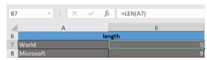
1. LEN()
The function LEN() returns the total number of characters in a string. So, it will count the overall characters, including spaces and special characters. Given below is an example of the Len function.
2. NOW()
The NOW() function in Excel gives the current system date and time.
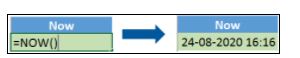
The result of the NOW() function will change based on your system date and time.
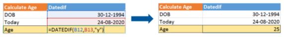
3. DATEDIF
The DATEDIF() function provides the difference between two dates in terms of years, months, or days.
Below is an example of a DATEDIF function where we calculate the current age of a person based on two given dates, the date of birth and today’s date.
4. VLOOKUP
Next up in this article is the VLOOKUP() function. This stands for the vertical lookup that is responsible for looking for a particular value in the leftmost column of a table. It then returns a value in the same row from a column you specify.
Below are the arguments for the VLOOKUP function:
lookup_value – This is the value that you have to look for in the first column of a table.
table – This indicates the table from which the value is retrieved.
col_index – The column in the table from the value is to be retrieved.
range_lookup – [optional] TRUE = approximate match (default). FALSE = exact match.
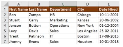
We will use the below table to learn how the VLOOKUP function works.
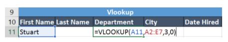
If you wanted to find the department to which Stuart belongs, you could use the VLOOKUP function as shown below:
Here, A11 cell has the lookup value, A2: E7 is the table array, 3 is the column index number with information about departments, and 0 is the range lookup.
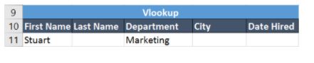
If you hit enter, it will return “Marketing”, indicating that Stuart is from the marketing department.
5. HLOOKUP
Similar to VLOOKUP, we have another function called HLOOKUP() or horizontal lookup. The function HLOOKUP looks for a value in the top row of a table or array of benefits. It gives the value in the same column from a row you specify.
Below are the arguments for the HLOOKUP function:
- lookup_value – This indicates the value to lookup.
- table – This is the table from which you have to retrieve data.
- row_index – This is the row number from which to retrieve data.
- range_lookup – [optional] This is a boolean to indicate an exact match or approximate match. The default value is TRUE, meaning an approximate match.
Given the below table, let’s see how you can find the city of Jenson using HLOOKUP.
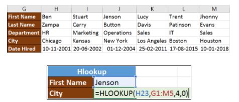
Fig: Hlookup function in Excel
Here, H23 has the lookup value, i.e., Jenson, G1:M5 is the table array, 4 is the row index number, 0 is for an approximate match.
Once you hit enter, it will return “New York”.
6. IF
The IF() function checks a given condition and returns a particular value if it is TRUE. It will return another value if the condition is FALSE.
In the below example, we want to check if the value in cell A2 is greater than 5. If it’s greater than 5, the function will return “Yes 4 is greater”, else it will return “No”.
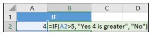
Fig: If function in Excel
In this case, it will return ‘No’ since 4 is not greater than 5.
‘IFERROR’ is another function that is popularly used. This function returns a value if an expression evaluates to an error, or else it will return the value of the expression.
Suppose you want to divide 10 by 0. This is an invalid expression, as you can’t divide a number by zero. It will result in an error.
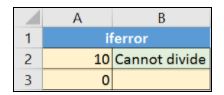
The above function will return “Cannot divide”.
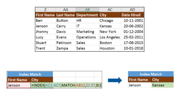
7. INDEX-MATCH
The INDEX-MATCH function is used to return a value in a column to the left. With VLOOKUP, you’re stuck returning an appraisal from a column to the right. Another reason to use index-match instead of VLOOKUP is that VLOOKUP needs more processing power from Excel. This is because it needs to evaluate the entire table array which you’ve selected. With INDEX-MATCH, Excel only has to consider the lookup column and the return column.
Using the below table, let’s see how you can find the city where Jenson resides.
Now, let’s find the department of Zampa.

8. COUNTIF
The function COUNTIF() is used to count the total number of cells within a range that meet the given condition.
Below is a coronavirus sample dataset with information regarding the coronavirus cases and deaths in each country and region.

The COUNTIFS function counts the number of cells specified by a given set of conditions.
If you want to count the number of days in which the cases in India have been greater than 100. Here is how you can use the COUNTIFS function.

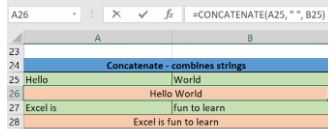
9. CONCATENATE
This function merges or joins several text strings into one text string. Given below are the different ways to perform this function.
- In this example, we have operated with the syntax =CONCATENATE(A25, ” “, B25)
- In this example, we have operated with the syntax =CONCATENATE(A27&” “&B27)
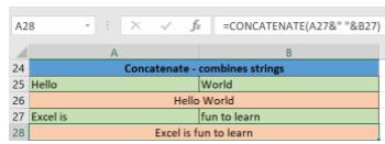
Those were the two ways to implement the concatenation operation in Excel.
10. FLOOR
Contrary to the Ceiling function, the floor function rounds a number down to the nearest multiple of significance.
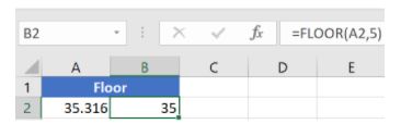
Fig: Floor function in Excel
The nearest lowest multiple of 5 for 35.316 is 35.