A scatter plot is a type of data visualization that displays values for two variables as a collection of points on a two-dimensional graph. Each point represents an observation from the dataset, with the position on the x-axis corresponding to one variable and the position on the y-axis corresponding to the other variable. Scatter plots are particularly useful for showing the relationship or correlation between the two variables, identifying trends, clusters, and outliers.
Key Features of a Scatter Plot:
- X-Axis and Y-Axis: Represent two different variables. The choice of which variable to place on which axis can depend on the context or the specific analysis being performed.
- Points: Each point on the scatter plot represents an individual observation from the dataset. The coordinates of the point correspond to the values of the two variables.
- Correlation: Scatter plots can reveal correlations between the variables:
- Positive correlation: As the value of one variable increases, the value of the other variable also increases.
- Negative correlation: As the value of one variable increases, the value of the other variable decreases.
- No correlation: There is no discernible pattern or relationship between the variables.
- Trend Line (Optional): Sometimes a trend line (or line of best fit) is added to the scatter plot to summarize the relationship between the variables.
- Clusters: Scatter plots can help in identifying clusters or groups of data points that are close to each other, suggesting similar behavior or characteristics.
- Outliers: Points that are far away from other points can be easily identified as outliers, which may require further investigation.
Example code:
import matplotlib.pyplot as plt
import seaborn as sns
import pandas as pd
import numpy as np
# Sample DataFrame
np.random.seed(42)
n = 100
df = pd.DataFrame({
‘x’: np.random.randn(n) * 10 + 50, # Random data for x-axis
‘y’: np.random.randn(n) * 20 + 100, # Random data for y-axis
‘category’: np.random.choice([‘A’, ‘B’, ‘C’], n), # Random categories
‘size’: np.random.rand(n) * 500 + 100, # Random sizes
‘color’: np.random.rand(n) # Random color values
})
# Scatter Plot
plt.figure(figsize=(14, 8))
scatter = sns.scatterplot(
data=df,
x=’x’,
y=’y’,
hue=’category’, # Color by category
size=’size’, # Size by a continuous variable
palette=’coolwarm’, # Custom color palette
sizes=(50, 500), # Scale the sizes
edgecolor=’black’, # Edge color for points
alpha=0.7 # Transparency
)
# Add annotations for a few points
for i in range(0, n, 10): # Annotate every 10th point
plt.text(
df[‘x’][i],
df[‘y’][i],
f'({df[“x”][i]:.1f}, {df[“y”][i]:.1f})’,
horizontalalignment=’center’,
size=’medium’,
color=’black’,
weight=’semibold’
)
# Title and labels
plt.title(‘Scatter Plot Example’, fontsize=18)
plt.xlabel(‘X-axis Label’, fontsize=14)
plt.ylabel(‘Y-axis Label’, fontsize=14)
# Customize the legend
plt.legend(title=’Category’, bbox_to_anchor=(1.05, 1), loc=’upper left’)
# Show plot
plt.grid(True)
plt.tight_layout()
plt.show()
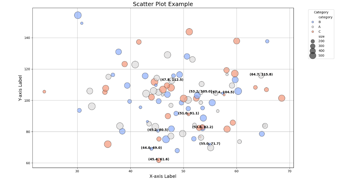
example output: